
Supply is quite a straightforward concept, understood by non-economists and economists alike. The term “supply” refers to the amount of a good or service that a firm is willing and able to offer for sale for a given period of time. For a slightly unexpected example, consider the labor market: the supply of labor is the amount of time per week, month, or year that individuals are willing to spend working, as a function of the wage rate (keep reading to understand how, exactly, the supply of labor is linked to the wage rate).
The Law of Supply
The law of supply is the direct relationship between price and quantity supplied. It is one of the two most fundamental laws in the field of economics (along with the law of demand).
The law of supply states the following: as the quantity of a good or service supplied increases (i.e. the amount available for sale increases), the price of that good or service also increases; likewise, as the price of that good or service increases, its quantity offered by suppliers will also increase.
Why is this the case?
Simply put, it’s a rule across the board that firms and other suppliers will always seek to sell their goods and services at maximum profit. So, when the price of those goods and services increases, suppliers will increase the amount of them that they’re selling, which should allow them to make a greater profit. In other words, the positive correlation between price and quantity supplied is based on the potential increase in profitability that occurs with an increase in price.
Nearly all goods and services follow the law of supply. This makes intuitive sense: of course, firms will want to produce and sell greater quantities of whichever item makes them the most money.
To put the law of supply another way: if every other factor remains the same, then an increase in the price of a good or service results in an increase in the quantity supplied of that good or service. This positive relationship is the reason for the supply curve sloping upwards (more on that below).
How the law of supply relates to the law of demand
Contrast the law of supply with the related law of demand (of course, you often hear them paired together, as “supply and demand”). The law of demand states something similar but distinct: that demand will decrease when the price of a good rises, and when the price decreases, demand increases. The law of supply and the law of demand provide a clear window into the way that resources are allocated and prices are set within a competitive free market economy. Anyone who wants to understand how economics work must have a firm grasp of these two fundamental laws.
The Supply Curve
The supply curve (SC) is a visual, mathematical method for illustrating the relationship between the price of a product, and the quantity of the product businesses are willing to sell at that price. It slopes in an upward direction from the left to the right, for the quite simple reason that both the quantity supplied and the price of the good/service increase when the other variable increases.
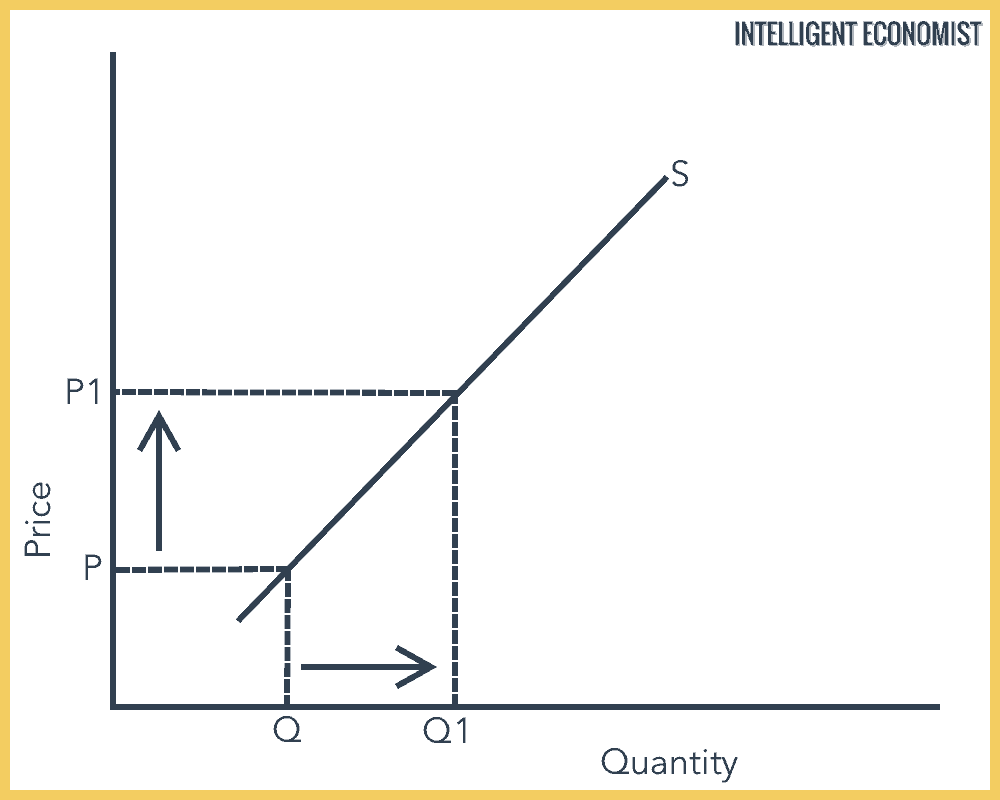
The standard form of the supply curve shows the quantity of the good/service supplied on the horizontal axis (x-axis) at the bottom of the graph, and the price of that good/service on the vertical axis (y-axis), to the left of the image. (Please note that this does not mean that the quantity is the dependent variable, and the price is the independent variable. This would be true in many other fields, in which the x-axis normally shows the independent variable and the y-axis typically shows the dependent variable, but this is not generally the case in economics.)
Additionally, the supply curve isn’t absolutely required to be drawn as a simple straight line; however, you’ll usually see it drawn as a straight line because it’s easier both to draw and to comprehend. Take a look at the illustration below to get an idea of how supply curves work:
Movement Along The Supply Curve
A movement along the curve only occurs if there is a change in quantity supplied caused by a change in the good’s own price. For example, if the price increases from P to P1, then the quantity supplied increases from Q to Q1 (see the graphic above for reference). The movement along the supply curve is affected by the price and the quantity supplied.
The Mathematical Equation for the Supply Curve
Naturally, it’s possible to write the supply curve out as an algebraic equation. In general, you’ll find that the supply curve is written out as quantity supplied (Qs) as a function of price. The reverse is the price (P) as a function of the quantity supplied—this is known as the inverse supply curve, and is less common. Here are the equations for these two variants:
Supply Curve: Qs = -3 + (3/2) P
Inverse Supply Curve: P = 2 + ⅔ Qs
You can plot equations for the supply curve (it’s really not terribly difficult!), and if you do so, it should come out looking something like the graph illustration we provided above. To make the process of plotting the equation easier, note the location on the point that goes across the price axis, which is equivalent to where demand quantity is 0 (written out algebraically, this means 0 = -3 + (3/2)P); you can see in that equation that if you solve for P, you get 2—P is equal to 2.
Why Does a Supply Curve Slope Upward?
A supply curve slopes upward because, for producers, increases in the price of a good or service incentivize a higher quantity of production. The x-axis indicates quantity supplied and the y-axis indicates price; as the price increases, the profit potential of selling products likewise increases. That higher possible profit means producers will earn more money for each unit of that good or service (as long as other important details about the product such as cost of production and demand remain the same), so producers are motivated to produce more.
Assuming that the economy lacks any confounding factors that might prevent it from being absolutely competitive (in other words, in an ideal economy), this is how any producer or firm will respond to such a situation. In reality, because no economy is perfectly competitive, the behavior and decision-making of firms are likely to be a bit more complex than this, and not as consistent as expected.
Another factor in the upward slope of a supply curve is the law of diminishing returns. This idea describes the way in which output is affected when firms use more variable inputs while maintaining one or more factors of production as fixed. In general, this fixed factor of production is likely to be real capital (for instance, machinery, equipment, buildings, and so forth). With additional, variable factors of production (commonly labor), the marginal returns (that is, additional output) for each additional unit of input will eventually diminish.
Determinants Of Supply
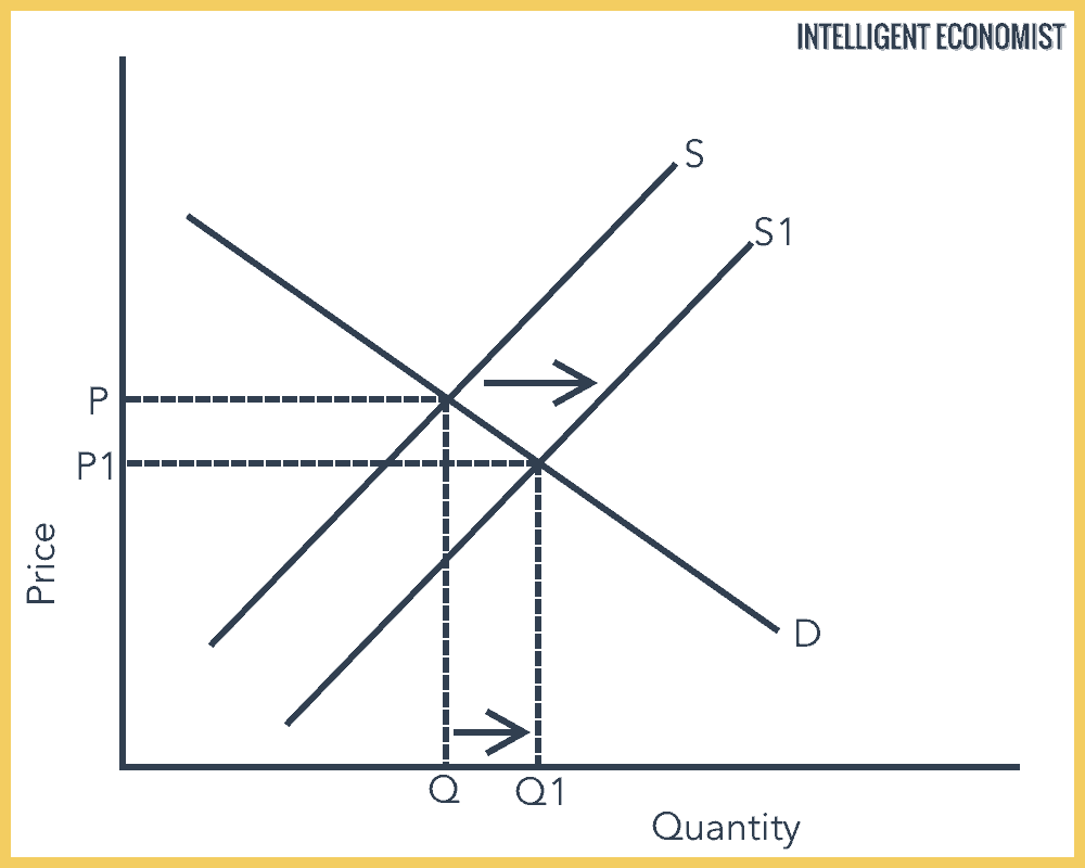
A shift in the supply curve, referred to as a change in supply, occurs only if a non-price determinant of supply changes. For example, if the price of an ingredient used to produce the good, a related good, were to increase, then the supply curve would shift left. The following factors affect supply (S), so changes in these determinants will shift the supply curve.
1. Input prices
If the price of raw materials used in the production of a product goes down, then S will increase—this means that it will shift to the right. And in the reverse, if the price of inputs increases, then S will decrease, meaning that it will shift to the left.
2. Improvements in technology
If there are any major advancements in technology, then production becomes more efficient and the cost of production almost certainly decreases. This means, then, that S shifts to the right. For example, USB flash drives began with a storage capacity of 8 MB. These early versions were fairly expensive, and storage wasn’t terribly extensive. Now with steady improvements, you can actually buy flash drives with hundreds of GB of capacity at a lower price—with technological advancements, these and so many other items function better AND typically decrease in cost, making this a win-win for consumers.
3. Government policy
Government policies can have a significant impact on supply. For example: if the government imposes a subsidy on the good, then S increases (which is the government’s intention in the case of a subsidy), while a tax on the good will have the opposite effect of decreasing S.
4. Size of the market
If the size of the market increases, then it is quite likely that there will be an increase in the number of firms in the market. With more sellers now participating in the market, this tends to increase S overall. A lot of people might think that more sellers being in the market will prompt each of the sellers to produce less—and that makes sense, at first thought. However, in reality, this doesn’t tend to occur in a market that contains a healthy and normal level of competition.
5. Time
This might seem like an unexpected one, but think about it—over time, firms can increase capacity (i.e. of production or providing a service). Increasing capacity means having the ability to increase S.
6. Expectations
The concern about future market conditions and the status of future determinants of supply can directly affect S. If the seller believes that the demand for his product will sharply increase in the foreseeable future, then the firm owner may immediately increase production in anticipation of future price increases. This increase in production would shift the supply curve outwards, which means that it is also increasing supply.