Budget Constraint

When consumers’ income limits their consumption behaviors, this is known as a budget constraint. In other words, it’s all of the many combinations of goods/services that consumers are able to purchase in light of their particular income as well as the current prices of these particular goods/services.

In the short term, budget constraints can be reduced through the use of loans; however, analyzing budget constraint, in the long run, reveals that it is primarily governed by income, rent, and other more long-term factors.

Budget constraint constitutes the primary part of the concept of utility maximization. This concept can be summed up in the following question: “What affordable set of goods/services will maximize my happiness?” The word “affordable,” here, is linked to budget constraint. Meanwhile, “happiness” is linked to indifference curves.

A notable practical application of this concept is its use in the field of consumer theory, as a tool to examine the parameters of consumer choices.

Contents show

Calculating Budget Constraint

Economists will often reduce mathematical representations of budget constraint to a discussion of two goods at a time, so that the concept can be represented clearly on a graph with x-and y-axes.

Let’s use an example of these two goods. We’ll say the first is juice and the second is bread. Juice (PJuice) is $3 and bread (PBread) is $4. Meanwhile, the consumer has a total of $36 to spend (Income) on these two products. Additionally, the amount spent on juice is noted as 3J (J being the number of bottles of juice purchased), while the amount spent on bread is noted as 4B (B being the number of loaves of bread purchased). Budget constraint is represented by the combined amount of both juice and bread that one can spend within that total available income limit of $36. See below for a simpler representation of this example.

P_Juice = $3

P_Bread = $4

Income available = $36

Amount spent on juice = 3J

Amount spent on bread = 4B

Total spending = 3J + 4B

Budget constraint: 4B + 3J = $36

The Budget Constraint Equation

Here’s the equation itself. This equation applies to most budget constraint calculations, assuming there are no extra factors (e.g. rebates, volume discounts, and so forth).

P_XX + P_YY = I

This formula might seem confusing at first glance, but it’s actually pretty straightforward once you get the hang of it. It’s saying that the price of the good on the x-axis multiplied by that same good’s quantity, plus the price of the good on the y-axis multiplied by its own quantity, is equal to income.

Additionally, the budget constraint’s slope is the negative of the of the x-axis good’s price divided by the y-axis good’s price. With this, keep in mind that slope is typically defined as the change in y over (divided by) the change in x, but it’s actually a bit different than that.

Budget Constraint Graph

Step 1: Determine where the budget constraint touches each axis

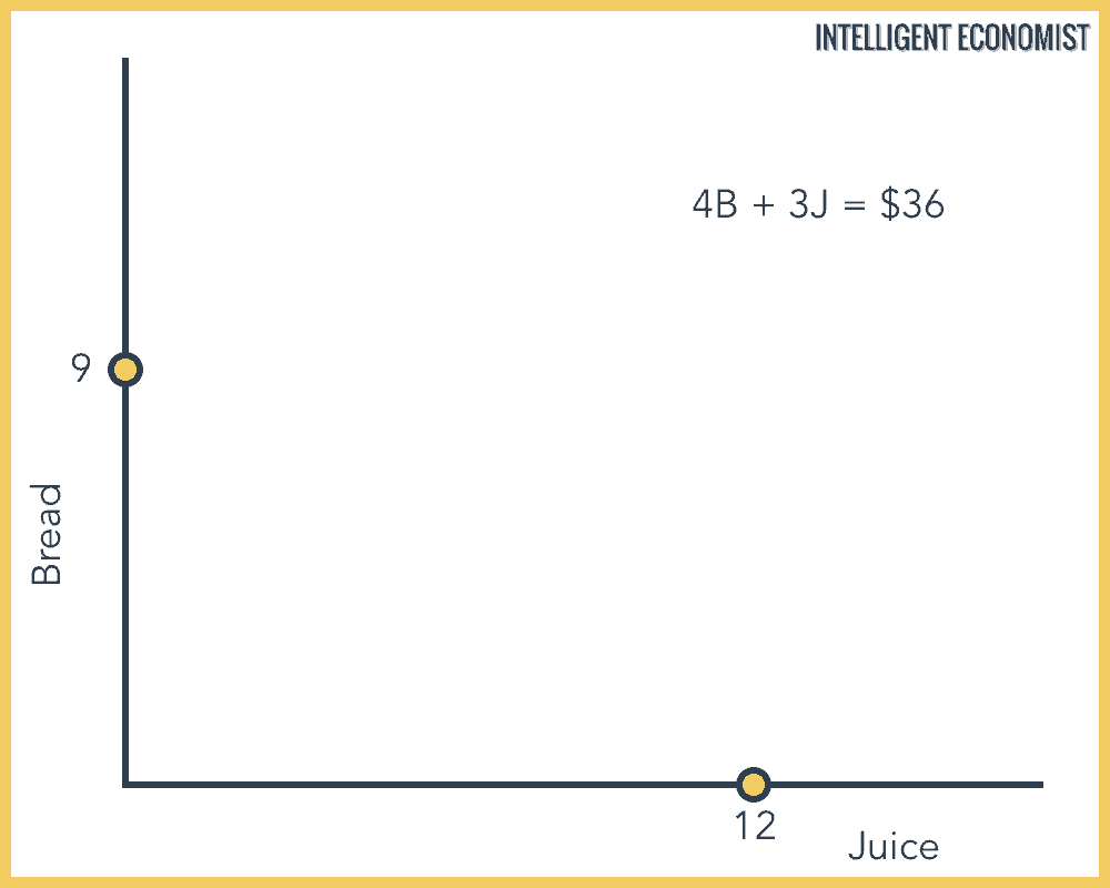
It’s helpful to begin by determining where it touches the x- and y-axes. You can figure that out by deciding how much of each of the goods the consumer could purchase if they only spent their available income on that good. In our example, if the hypothetical consumer only spent their $36 on bread, they’d be able to buy 9 loaves of bread (because 36 ÷ 4 = 9). On the graph, this appears as the point (0, 9). But if instead, they only spent their $36 on juice, they could purchase 12 bottles of juice (because 36 ÷ 3 = 12). On the graph, this appears as the point (12, 0).

Step 2: Add a line and determine its slope

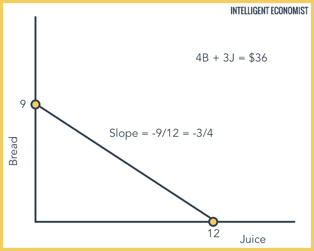
Next, you draw the budget constraint onto the graph as a line, by directly connecting the two points created during step 1. Then you have to determine the slope of this line. To calculate the slope of a line, divide the change in y by the change in x. In this case, you have -9 ÷ 12, which is reduced to -3/4. That’s the slope. What this actually means, in terms of budget constraint for this example, is that 3 juices must be sacrificed to purchase 4 loaves of bread.

Step 3: Interpret the graph

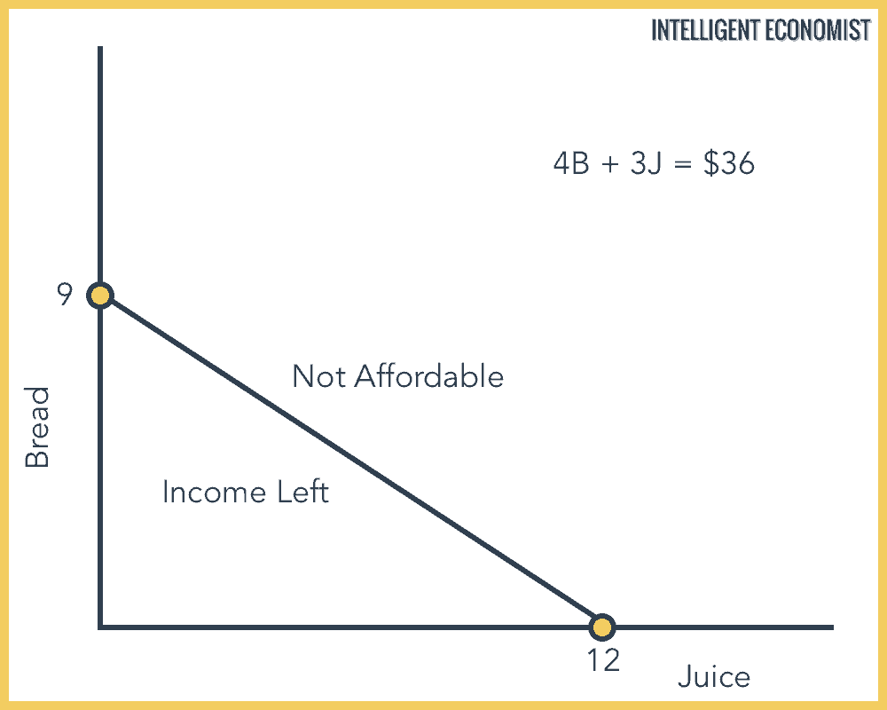
Budget constraint is represented by all the points on the graph at which the consumer uses the entirety of their available income on purchases of these goods. All points from the origin (0,0) to the budget constraint line are those at which the consumer doesn’t spend their entire income. Meanwhile, all the points beyond the budget constraint line on the graph above are the amounts of purchases that the consumer can’t afford.

Sunk costs aren’t Factored into Budget Constraint

The concept of budget constraint doesn’t account for sunk costs. Sunk costs are costs already received in the past that can’t be changed in the present. When you’re working with the budget constraint framework, you’re not expected to consider sunk costs as part of the present economic decision.

For instance, if you spend money on a ski trip, and then realize that you hate skiing once you’ve already paid for it, the cost of the trip is now a sunk cost. You might finish the ski trip (e.g., spend the three more days left) to feel like you haven’t wasted your money. But here’s the problem: now you’re paying an opportunity cost by spending those three days doing something you hate instead of something you enjoy. Why waste your time?

If you think about things in terms of budget constraint, you effectively acknowledge that the sunk costs are unchangeable and it’s better to make decisions in light of your future preferences, rather than your desire to not have wasted money. This is something of philosophical consideration.